Block 1 · Fundamentals of Decompression
How your body takes up gases — and lets them go again
Introduction
This block lays the foundation for everything that follows: how inert gas gets into the body, how it leaves again, and why we use mathematical models (e.g. Bühlmann) to plan ascent profiles. This is not about formulas, but about relationships — and what they mean in practice. We’ll work with the core ideas behind Bühlmann-style models (compartments, half-times, M-values) and how they are modified by Gradient Factors. You’ll understand how to apply them — and where the limits and uncertainties are.
Before we get into decompression, a quick reminder of the most basic gas laws.
On-gassing and off-gassing
As soon as you descend, ambient pressure increases — and with it the partial pressure of inert gases in your breathing gas. In the lungs, inert gas diffuses into the blood and is carried throughout the body. If the inert-gas pressure in the blood is higher than in the surrounding tissues, gas diffuses into those tissues. If the inert-gas pressure in the blood is lower, gas leaves the tissues again and can be eliminated via the lungs.
On-gassing: what changes under pressure?
The basic principle behind on-gassing and off-gassing is Henry’s Law. Whenever a gas borders a liquid — or different tissues border each other — partial pressures will tend to equalise over time. During descent, ambient pressure increases, and with it the nitrogen partial pressure in the breathing gas. That drives increased inert gas uptake. During ascent, pressure drops again — and the gas has to leave the body. You can watch that process more closely in the animation.
Tissue compartments and half-times
In reality, different tissues take up and release inert gas at very different speeds.
We can’t calculate that for every organ individually.
That’s why models use artificial “compartments”:
each one is assigned a half-time, and together they cover the full spectrum of human tissues.
The half-time describes how long a compartment needs to adapt halfway to a new pressure situation.
Example: a 5-minute half-time → after 5 minutes it’s at 50%, after 10 minutes at 75%, after 15 minutes at 87.5%.
The most commonly used model today, the Bühlmann ZHL-16C algorithm, uses 16 model tissues with half-times between 5 and 635 minutes.
You can explore how saturation develops in these tissues over time in the next tool.
Saturation in a single model tissue
We now have the building blocks: tissues on-gas, they do so at different speeds, and as pressure decreases, they off-gas again.
To talk about off-gassing — and about limits of supersaturation — this plot is a very helpful mental model.
It makes saturation and, especially, off-gassing in a model tissue easy to see.
Part 1: How is the plot constructed?
Part 2: How can we track saturation and desaturation – and what limits are we talking about?
With this basic picture in mind, you’re well prepared for the next section: the limits of supersaturation.
↑ Back to topLimits of supersaturation: M-values and Gradient Factors
Because we can’t directly look inside the body, decompression models exist.
They aim to represent the processes as plausibly as possible and provide a workable estimate of risk.
The most widely used model is the Bühlmann ZHL-16C algorithm, which we’ll use here to explain the concepts.
We’ve already seen the central question behind all decompression theory:
how supersaturated can a tissue become before the risk of DCS becomes unacceptably high?
That’s exactly what M-values — and their modification via Gradient Factors — are about.
M-values
Each model tissue has a limit for how much inert-gas supersaturation it can tolerate. That limit is what an M-value represents.
The M-value is the inert-gas pressure a tissue can “just about tolerate” at a given ambient pressure.
If it is exceeded, the risk of DCS symptoms increases.
M-values differ between model tissues. The model assumes that fast tissues can tolerate higher supersaturation than slow tissues.
And M-values are depth-dependent. An M-value always consists of the current ambient pressure plus the tolerated supersaturation.
At higher ambient pressure, the Bühlmann model also allows a higher tolerated supersaturation.
In other words: it assumes that a higher overpressure is tolerated at depth than at the surface.
What does this look like in practice for a single model tissue — in terms of M-values, no-decompression limits, and decompression? Let’s go back to our off-gassing plot.

We’ve already seen that the risk of DCS increases the further a tissue moves into the supersaturation range.
You can never predict exactly when a given person will develop symptoms.
You can only estimate a general statistical risk — and then choose a limit based on that.
That’s what M-values do: they define a boundary for an “acceptable” level of risk.
Even though an M-value is an exact number (down to several decimal places), it does not represent a sharp, natural boundary.
It’s a hard line drawn into a fuzzy zone where risk gradually increases.
For each model tissue, these M-values form an M-line that limits ascent.
If a tissue is only saturated to the point where an ascent would not cross that M-line, the dive is considered a no-decompression dive.
Once the boundary would be crossed, decompression stops are needed to allow some off-gassing already during the ascent.
By the time you reach the surface, the boundary should no longer be exceeded.
M-values and the no-decompression limit
“No-decompression” means: a direct ascent would not exceed any M-value.
That doesn’t eliminate risk, but it keeps it within a range the model defines as acceptable.
At different depths, different tissues are the first to reach their maximal tolerated load and therefore end the no-deco time.
In this tool you can see, for each depth, which tissue is limiting.
If you explore which tissue reaches a critical inert-gas pressure first at different depths, you’ll notice the following:
On deep dives, around 40 m, the no-decompression limit is reached quickly — because the fastest tissue would hit its M-value on a direct ascent.
At more moderate depths, the “leading tissue” shifts: the tissue that comes closest to its M-value during ascent changes to higher-numbered compartments.
The fastest tissues tolerate such high supersaturation that at 20 m they can be fully saturated without that being critical.
The animation stops when the original Bühlmann M-values are reached.
Of course you can exceed that boundary — then you’ll need to plan stops during the ascent to give the most supersaturated tissues time to off-gas a bit.
And of course you can modify M-values, shifting no-deco limits or extending decompression.
Gradient Factors
Gradient Factors are a way to modify M-values and build an additional safety buffer.
To understand how they work, we’ll return once more to our basic plot of off-gassing in a model tissue.
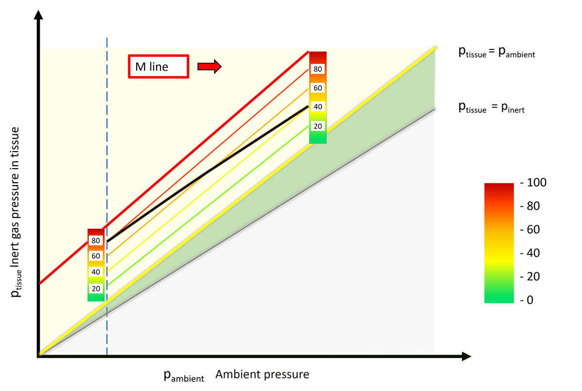
Below the original M-line you can see additional lines: the modified M-lines. If you consider the original M-values too risky (which is today’s general consensus), you can simply reduce the amount of supersaturation you are willing to accept. That is done as a percentage of the tolerated supersaturation: you draw a new line at 80%, 60%, or even less.
If you stick to one shifted line, you’ve simply added extra conservatism.
In practice, two Gradient Factors are commonly used: GF Low and GF High.
This is usually written as, for example, GF 40/80 — the first number is GF Low, the second is GF High.
Why do this? Historically, this practice comes from the idea that deeper stops during ascent might help control bubble growth.
How sensible that is is discussed in the block on current research.
With a lower GF Low, you move slowly during ascent from the lower GF towards the higher GF.
GF Low largely determines the depth of the first stop; GF High determines the level of supersaturation at the surface.
Choosing Gradient Factors
Keeping an eye on all tissues: dive planning
Up to this point we’ve mostly looked at what happens in a single model tissue, and used that to define limits of supersaturation.
But the model works with 16 tissues with very different properties — so during ascent we have to keep all of them in view.
The no-deco finder has already shown that different tissues become limiting at different depths.
What applies to no-deco time also matters in decompression: the tissue that comes closest to its M-value can change during ascent.
We need a way to watch all model tissues at the same time.
Heatmaps offer exactly that kind of visualisation.
To keep the entry as simple as possible, here’s a very basic deco planner that shows the profile and a heatmap.
You can enter one or more depths and times, choose your breathing gas and your GFs.
When you hit calculate, you’ll get the dive profile, the heatmap, and a runtime.
The heatmap shows saturation of each tissue in shades of blue: the darker it gets, the closer the tissue is to being saturated.
During ascent the tissues move into the supersaturation range, shown here in traffic-light colours.
Green means a very low gradient; red means 100% of the M-value is reached.
For real dive planning, you should use a properly validated planner.
But here you can clearly see what changes when you shift your Gradient Factors.
Full dive-planning practice is covered in Block 6.
Finished playing with the planner? Then try to see if you can recognise which profiles and heatmaps belong together.